Simulating Mancala, part 1
The code used for all simulations and analysis described in this post can be found on my github
A few years ago, my partner introduced me to the board game mancala, also known as Kalaha. I have always suspected that there is an advantage to whoever moves first. Let’s see if we can test this hypothesis with python!
Rules
Mancala is a two-player board game, where players compete to capture more marbles than their opponent. The rules are as follows:
- Each player has six buckets, initially containing four marbles. They also have a score bucket.
- A move is made by player one choosing one of their six buckets, collecting all their marbles.
- The player then distributes the marbles in subsequent buckets, including the player’s score bucket, moving in an anti-clockwise direction until no marbles remain.
- The opponent’s score bucket is skipped over.
Depending on the bucket that a player places their last marble in, additional rules are applied:
- If the player ends in a non-zero bucket, then they collect the stones in that bucket and continue moving anti-clockwise around the board.
- If the player ends their turn in their score bucket, then they get to choose a new move from their non-zero buckets.
- If the player ends in an empty bucket, then the player’s turn is over.
- The game is over when either half of the marbles have been captured, or one player manages to empty all the buckets on their side.
- When the game is over, any remaining marbles on each player’s side are added to their score bucket.
The winner is the player with the most marbles.
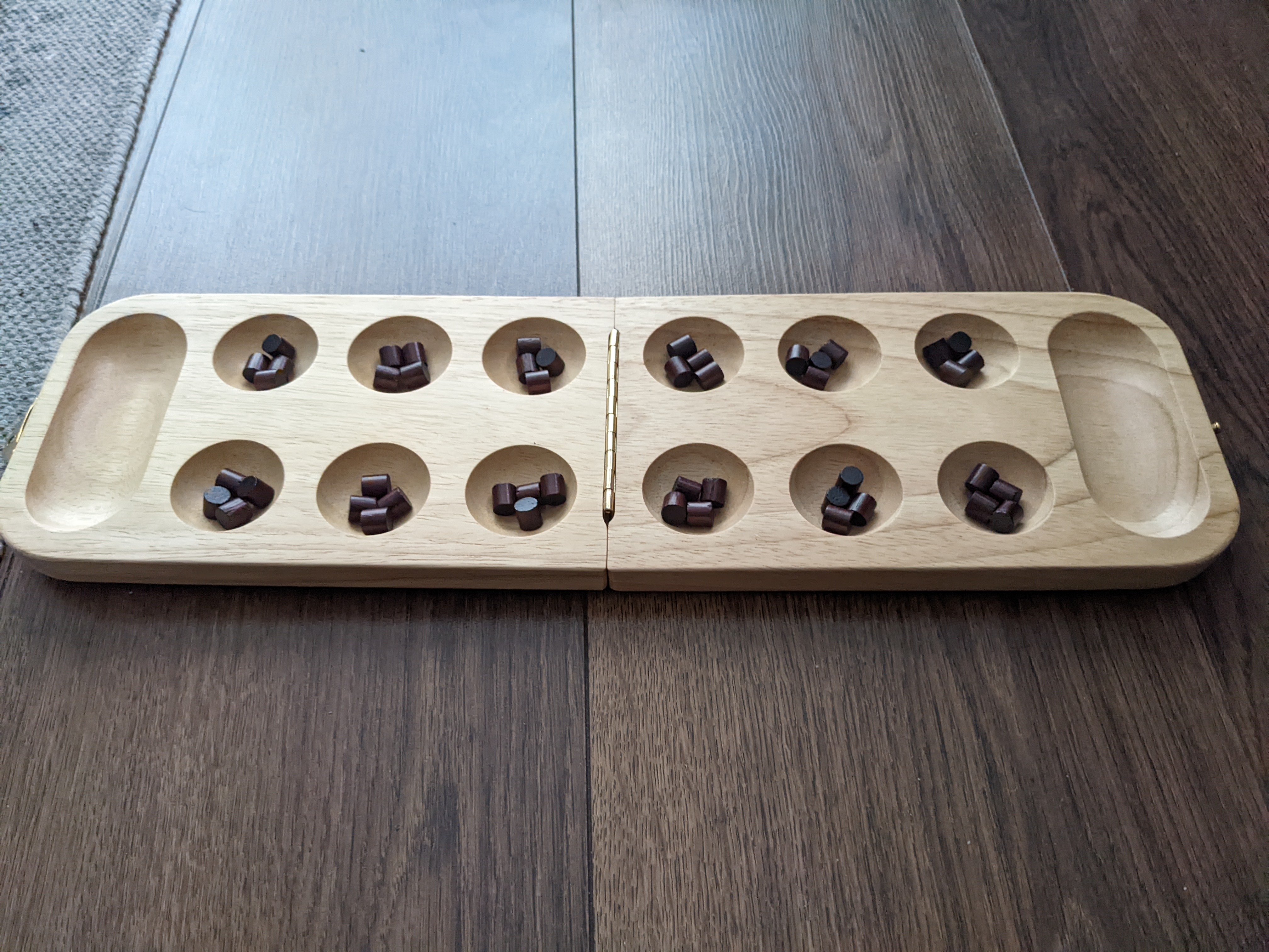
The board is represented like so:
from core.game.Board import Board
board = Board(n_start_marbles=4)
print(board)

'''
        4 4 4 4 4 4
[0]                      [0]
        4 4 4 4 4 4

'''

board.make_player_move(1, 3, 1) # makes a move for player 1, from bucket 3, on side 1
print(board)

'''
        4 4 4 4 4 4
[0]                      [1]
        4 4 0 5 5 5
'''
Initial analysis
Throughout the rest of this article, player one refers to the player who moves first, and player two is the player who moves second. Initially, I chose to simulate both players as a random agent. That is, from the available bucket choices a player has, one is selected randomly with equal weightings. As we will later see, this does not form an optimal strategy for either player.
For these tests, I ran 10000 simulations with player one and player two, utilising a random strategy for their move choice.
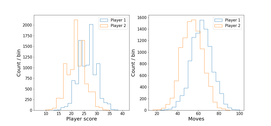
It’s clear that player one tends to have a higher score than player two, and thus we would expect player one to have a higher win percentage. Player one also makes more moves than player two, which is to be expected with the higher overall score that player one has. Examining the distribution of player moves for the three different outcomes (win, lose, draw) provides confirmation of this.
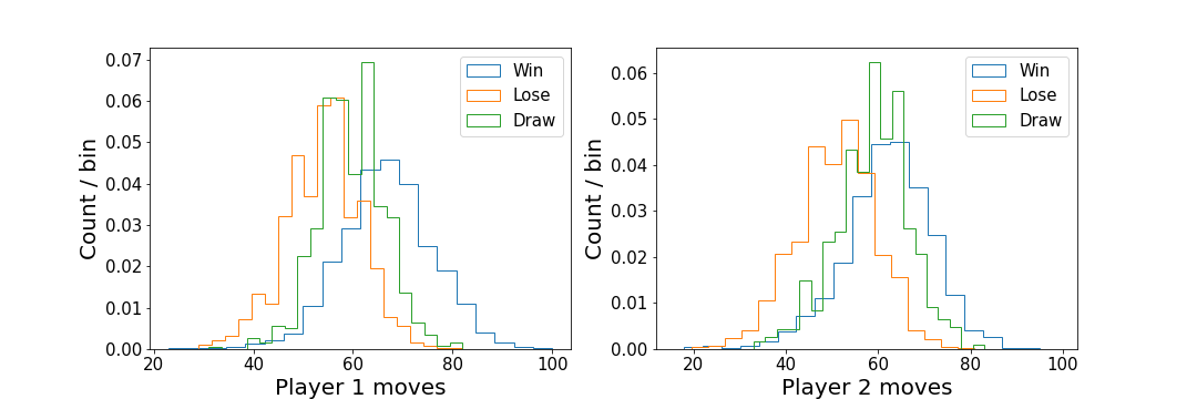
These distributions are unit normalised, to better compare the shapes.
When players win, the mean number of moves made is higher than the mean number of moves made when they lose. This might suggest that a selection strategy which maximises the number of moves made on a given turn could perform better than a random choice.
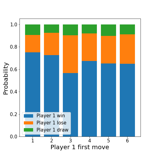
Because player one always moves first, with a free choice, it is interesting to calculate the win, lose, and draw rates for the different first move choices.
Different strategies
From the initial analysis, we know that players tend to win if they choose buckets which maximise the number of moves they make. Clearly, players using strategies which involve making choices maximising their score increase will also perform well. With these ideas in mind, we can develop different strategies for players to apply, and then simulate them against each other.
Exact strategy
For this strategy, the player makes choices by favouring moves which will end in the player’s goal, therefore giving them another move. If multiple moves of this kind are possible, they are played in order, starting with the closest to the player’s goal, enabling a repeated advantage of this rule.
from core.game.Board import Board
board = Board()
board.player_one_cups = [1, 3, 0, 3, 2, 1]
print(board)

'''
        6 6 6 6 6 6
[0]                      [0]
        1 3 0 3 2 1
'''

board.make_player_move(1, 6, 1)
board.make_player_move(1, 5, 1)
board.make_player_move(1, 4, 1)
print(board)

'''
        6 6 6 6 6 6
[0]                      [3]
        1 3 0 0 1 2
'''
If no such moves are possible, then the strategy falls back to either random, or a new strategy described below.
Max score strategy
For this strategy, the player chooses the bucket which will give them the largest score increase once all marbles have been distributed across the board. If a considered choice will result in the last marbles being place in the player’s goal, therein giving them another choice, then subsequent moves are considered in a recursive fashion.
Maximum marbles strategy
For this strategy, the bucket with the most marbles is chosen. If multiple moves fulfil this criteria, then a bucket is selected randomly, with equal probability.
Maximum moves strategy
Similar to the maximum score strategy, except that the figure of merit to be maximised is the number of moves a player will make.
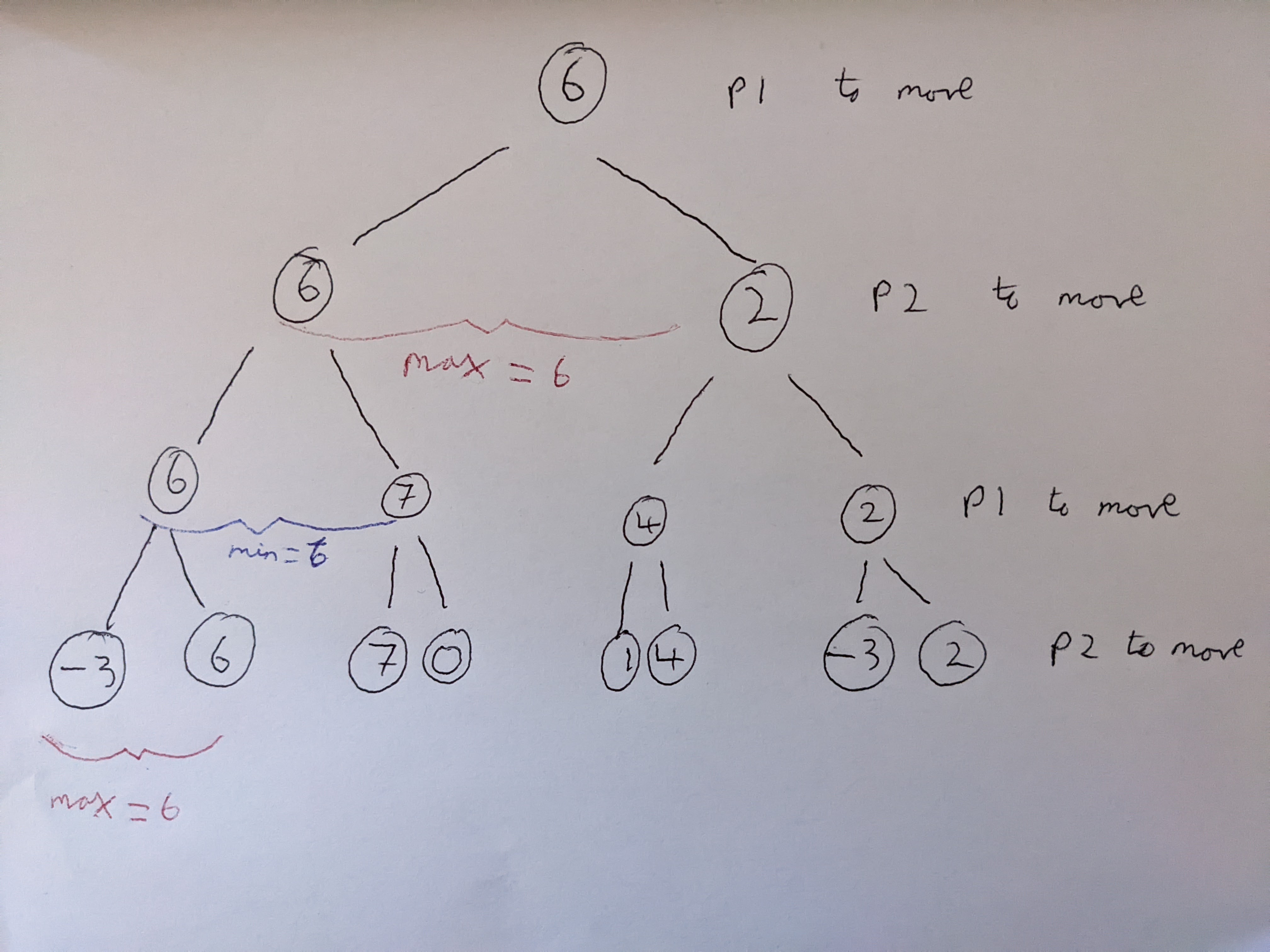
Minimax strategy
This strategy implements the so-called minimax strategy from game theory. A good explanation of this strategy that I found can be found in Sebastian Lague’s video.
After a full sequence of moves has been made, the board state is completely known for both players (i.e. moves are deterministic, and the players have perfect information). The evaluation of the current board state, can be written as the difference between player one’s score, and player two’s score. Player one will always try to maximise this evaluation, whereas player two will always try to minimise this evaluation.
If it is player one’s turn to move, then all of player one’s moves are considered, and the board evaluation after each of these moves is calculated. Then it will be player two’s turn to move, who will try to minimise the evaluation from their set of available moves. Player one will choose the move which gives the maximum evaluation of the set of these minima.
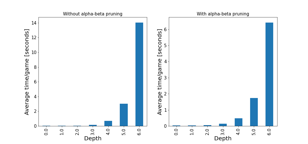
The tree depth is in theory unlimited, but in practice limited until the trees reach the end of the mancala game, or the computational time becomes too expensive. In my simulations, I set this to be 3, but investigated the computational time impact from higher depth values. One form of speed increase is alpha-beta pruning, which stops evaluating further move trees if no further improvement can be made. I.e. at least one alternative move which performs better than the move under consideration has been found. Some (not-so-quick) tests with different depth settings show that the average time per game (from 100 games) is much quicker with alpha-beta pruning applied.
The dependency of the depth parameter can be investigated by running 5000 simulations of player one (minimax) vs player two (max score).
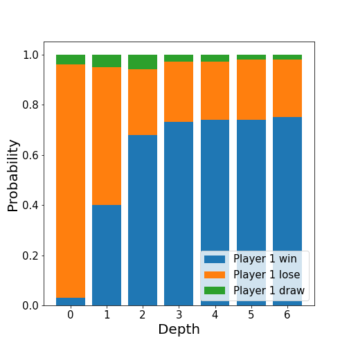
As we would expect, as the depth is increased, then player one’s win rate increases - to almost 80%! It appears that the win rate starts to saturate, which is likely because at some point the large depth means that the trees will reach the end of the game (no more moves will be available). However, I did not have the computational power (nor patience) to evaluate games with any higher depth.
Putting it all together
Putting it all together, I ran simulations of several different agents against each other, and calculated player one’s win rate for all these combinations. The matrix of these probabilities is shown below.
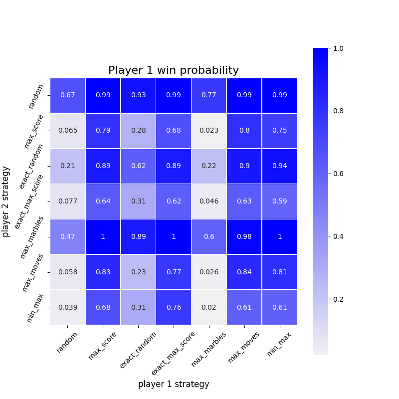
By inspecting the diagonal, we can answer my initial question; yes, it does appear that there is an advantage for the player moving first, provided that similar strategies are applied. It seems that most agents can out-perform random chance. I also investigated player one’s win rate dependency on the initial move choice.
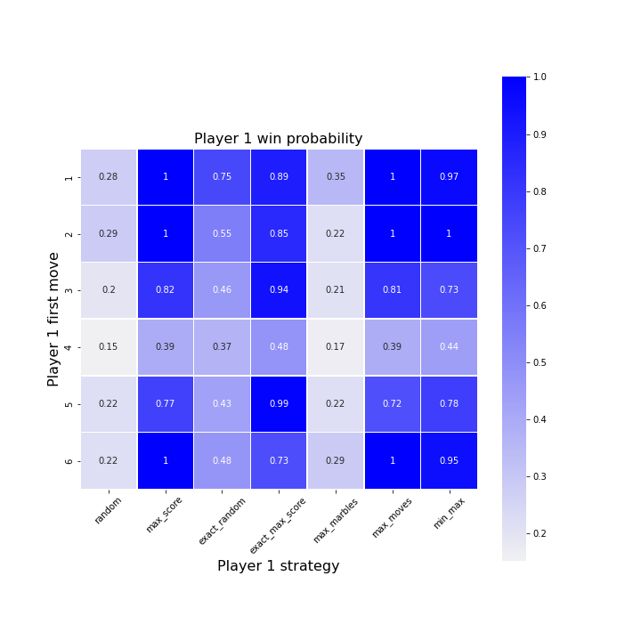
It appears that whatever the strategy, choosing bucket 4 as an initial choice is a bad idea.
What’s next?
This post has ‘part 1’ in the title…so what’s next? As an excuse to teach myselfreinforcement learning, I want to try implementing an agent with some sort of machine learning focus. When I find the time to do this, it will be described in a part 2.